Blog
26 Nov 2019 : Graphs of Waste, Part 3: A Continuously Differentiable Histogram Approach #
In part one we looked at how graphs can be a great tool for expressing the generalities in specific datasets, but how even seemingly minor changes in the choice of graphing technique can result in a graph that tells an inaccurate story.
In part two we found out we could draw a continuous line graph that captured several useful properties that are usually associated with histograms, notably that the area under the line graph is the same as it would be for a histogram between the measurement points along the $x$-axis.
But what if we want to go a step further and draw a smooth line, rather than one made up of straight edges? Rather than just a continuous line, can we present the same data with a continuously differentiable line? Can we do this and still respect this 'area under the graph' property?
It turns out, the answer is "yes"! And we can do it in a similar way. First we send the curve through each of the same points at the boundary of each column, then we adjust the height of the midpoint to account for any changes caused by the curvature of the graph.
There are many, many, ways to draw nice curves, but one that frequently comes up in computing is the Bézier curve. It has several nice properties, in that it's nicely controllable, and depending on the order of the curve, we can control to any depth of derivative we choose. We'll use second-degree Bézier curves, meaning that we'll be able to have a continuous line and a continuous first derivative. This should keep things nice and smooth.
Bézier curves are defined parametrically, meaning that rather than having a function that takes an $x$ input and produces a $y$ output, as is the common Cartesian case, instead it takes a parameter input $t$ that falls between 0 and 1, and outputs both the $x$ and $y$ values. In order to avoid getting confused with the variables we used in part two, we're going to use $u$ and $v$ instead of $x$ and $y$ respectively.
Here's the formula for a second-order Bézier curve.
$$
\begin{pmatrix} u \\ v \end{pmatrix} = (1 - t)^3 \begin{pmatrix} u_0 \\ v_0 \end{pmatrix} + 3(1 - t)^2 t \begin{pmatrix} u_1 \\ v_1 \end{pmatrix} + 3 (1 - t) t^2 \begin{pmatrix} u_2 \\ v_2 \end{pmatrix} + t^3 \begin{pmatrix} u_3 \\ v_3 \end{pmatrix} .
$$
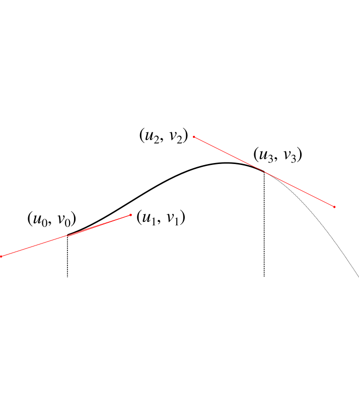
Where $\begin{pmatrix} u_0 \\ v_0 \end{pmatrix}$, $\begin{pmatrix} u_3 \\ v_3 \end{pmatrix}$ are the start and end points of the curve respectively, and $\begin{pmatrix} u _1\\ v_1 \end{pmatrix}$, $\begin{pmatrix} u_2 \\ v_2 \end{pmatrix}$ are control points that we position in order to get our desired curve.
The fact a Bézier curve is parametric is a problem for us, because it makes it considerably more difficult to integrate under the graph. If we want to know the area under the curve, we're going to have to integrate it, so we need a way to turn the parameterised curve into a Cartesian form.
Luckily we can cheat.
If we set $\begin{pmatrix} u_1 \\ v_1 \end{pmatrix}$ and $\begin{pmatrix} u_2 \\ v_2 \end{pmatrix}$ to be $\frac{1}{3}$ and $\frac{2}{3}$ of the way along the curve respectively, then things get considerably easier. In other words, set
\begin{align*}
u_1 & = u_0 + \frac{1}{3} (u_3 - u_0) \\
& = \frac{2}{3} u_0 + \frac{1}{3} u_3 \\
\end{align*}
and
\begin{align*}
u_2 & = u_0 + \frac{2}{3} (u_3 - u_0) \\
& = \frac{1}{3} u_0 + \frac{2}{3} u_3 .
\end{align*}
Substituting this into our Bézier curve equation from earlier we get
\begin{align*}
u & = (1 - t)^3 u_0 + 3 (1 - t)^2 t \times \left( \frac{2}{3} u_0 + \frac{1}{3} u_3 \right) + 3 (1 - t) t^2 \times \left( \frac{1}{3} u_0 + \frac{2}{3} u_3 \right) + t^3 u_3 \\
& = u_0 + t (u_3 - u_0) .
\end{align*}
When we choose our $u_1$ and $u_2$ like this, we can perform the substitution
$$
\psi(t) = u_0 + t(u_3 - u_0)
$$
in order to switch between $t$ and $u$. This will make the integral much easier to solve. We note that $\psi$ is a bijection and so invertible as long as $u_3 \not= u_0$. We can therefore define the inverse:
$$
t = \psi^{-1} (u) = \frac{u - u_0}{u_3 - u_0} \\
$$
It will also be helpful to do a bit of groundwork. We find the values at the boundary as
\begin{align*}
\psi^{-1} (u_0) & = 0, \\
\psi^{-1} (u_3) & = 1, \\
\end{align*}
and we also define the following for convenience.
$$
V(u) = v(\psi^{-1} (u)) .
$$
We'll use these in the calculation of the integral under the Bézier curve, which goes as follows.
$$
\int_{u_0}^{u_3} V(u) \mathrm{d}u
$$
Using the substitution rule we get
\begin{align*}
\int_{\psi^{-1}(u_0)}^{\psi^{-1}(u_3)} & V(\psi(t)) \psi'(t)\mathrm{d}t = \int_{t = 0}^{t = 1} v(\psi^{-1}(\psi(t))) (u_3 - u_0) \mathrm{d}t \\
& = (u_3 - u_0) \int_{0}^{1} v(t) \mathrm{d}t . \\
& = (u_3 - u_0) \int_{0}^{1} (1 - t)^3 v_0 + 3 (1 - t)^2 t v_1 + 3 (1 - t) t^2 v_2 + t^3 v_3 \mathrm{d}t \\
& = (u_3 - u_0) \int_{0}^{1} (1 - 3t + 3t^2 - t^3) v_0 + 3 (t - 2t^2 + t^3) v_1 + 3 (t^2 - t^3) v_2 + t^3 v_3 \mathrm{d}t \\
& = \frac{1}{4} (u_3 - u_0) (v_0 + v_1 + v_2 + v_3) .
\end{align*}
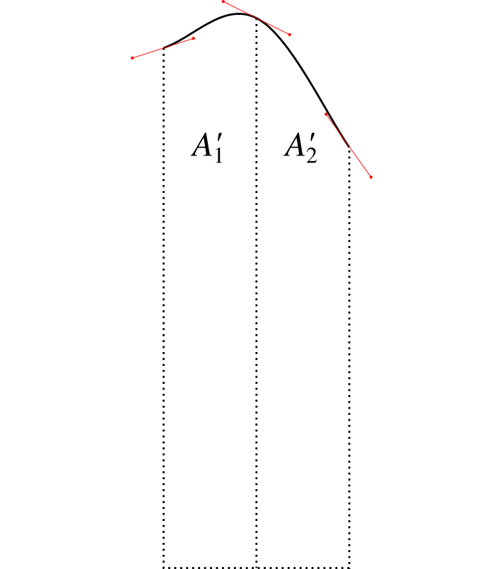
We'll bank this calculation and come back to it. Let's now consider how we can wrap the Bézier curve over the points in our graph to make a nice curve. For each column we're going to end up with something like this.
Now as before, we don't have control over $u_0$, $v_0$ because it affects the adjoining curve. We also don't have control over $u_1$ and $u_2$ because as just described, we have these set to allow us to perform the integration. We also must have $u_3$ set as $u_3 = u_0 + w / 2$ so that it's half way along the column.
Our initial assumption wil be that $v_3 = h$, but this is the value we're going to manipulate (i.e. raising or lowering the central point) in order to get the area we need. We shouldn't need to adjust it by much.
That just leaves $v_1$ and $v_2$. We need to choose these to give us a sensible and smooth curve, which introduces some additonal constraints. We'll set the gradient at the point $u_0$ to be the gradient $g_1$ of the line that connects the heights of the centrepoints of the two adjacent columns:
$$
g_1 = \frac{y - y_L}{x - x_L}
$$
where $x, y$ are the same points we discussed in part two, and $x_L, y_L$ are the same points for the column to the left. We'll also use $x_R, y_R$ to refer to the points for the column on the right, giving us:
$$
g_2 = \frac{y_R - y}{x_R - x} .
$$
Using our value for $g_1$ we then have
$$
v_1 = v_0 + g_1 (u_1 - u_0) .
$$
For the gradient $g$ at the centre of the column, we set this to be the gradient of the line between $y_1$ and $y_2$:
$$
g = \frac{y_2 - y_1}{x_2 - x_1} .
$$
We then have that
$$
v_2 = v_3 + g (u_2 - u_3) .
$$
From these we can calculate the area under the curve using the result from our integration calculation earlier, by simply substiuting the values in. After simplifying the result, we get the following.
$$
A_1' = \frac{1}{8}(x_2 - x_1) \left( 2y' + \frac{13}{6} y_1 - \frac{1}{6} y_2 + \frac{1}{6} g_1 (x_2 - x_1) \right)
$$
where $y'$ is the height of the central point which we'll adjust in order to get the area we need. This looks nasty, but it'll get simpler. We can perform the same calculation for the right hand side to get
$$
A_2' = \frac{1}{8}(x_2 - x_1) \left( 2y' + \frac{13}{6} y_2 - \frac{1}{6} y_1 - \frac{1}{6} g_2 (x_2 - x_1) \right) .
$$
Adding the two to give the total area $A' = A_1' + A_2'$ allows us to do a bunch of simplification, giving us
$$
A' = \frac{w}{2} \left( \frac{1}{2} y_1 + \frac{1}{2} y_2 + y' \right) + \frac{w^2}{48} (g_1 - g_2) .
$$
If we now compare this to the $A$ we calculated for the straight line graph in part two, subtracting one from the other gives us that
$$
y' = y + \frac{w}{24} (g_2 - g_1) .
$$
This tells us how much we have to adjust $y$ by to compensate for the area change caused by the curvature of the Bézier curves.
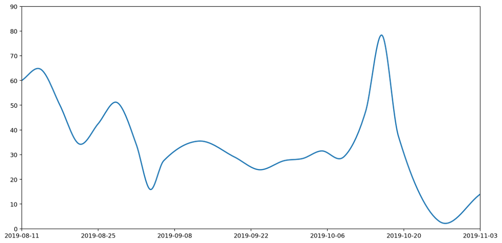
What does this give us in practice? Here's the new smoothed graph based on the same data as before.
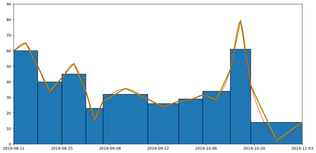
Let's overlay the three approaches — histogram, straight line and curved graphs — to see how they all compare. The important thing to note is that the area under each of the columns — bounded above by the flat line, the straight line and the curve respectively — are all the same.
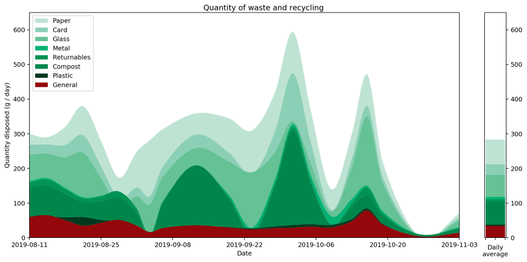
Because of the neat way Bézier curves retain their area properties, we can even stack them nicely, similarly to how we stacked our histogram in part one, to get the following representation of the full set of data.
Putting all of this together, we now have a pretty straightforward way to present area-under-the-graph histograms of continuous data in a way that captures that continuity. I call this graph a "histocurve". A histocurve can give a clearer picture of the overall general trends of the data. For example, each of the strata in the histocurve remains unbroken, compared to the strata in a classic histogram which is liable to get broken at the boundary between every pair of columns.
That's all great, but it's certainly not perfect. In the fourth and final part of this series which I hope to get out on the 3rd December, I'll briefly discuss the pitfalls of histocurves, some of their negative properties, and things I'd love to fix but don't know how.
Comments
Uncover Disqus comments